Using
Quickstart
An example dataset is available at data/berlin. You can reconstruct it using by running:
bin/opensfm_run_all data/berlin
This will run the entire SfM pipeline and produce the file data/berlin/reconstruction.meshed.json as output. To visualize the result you can start a HTTP server running:
python -m SimpleHTTPServer
and then browse http://localhost:8000/viewer/reconstruction.html#file=/data/berlin/reconstruction.meshed.json You should see something like
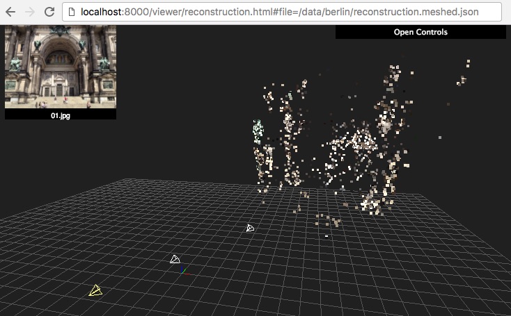
You can click twice on an image to see it. Then use arrows to move between images.
If you want to get a denser point cloud, you can run:
bin/opensfm undistort data/berlin
bin/opensfm compute_depthmaps data/berlin
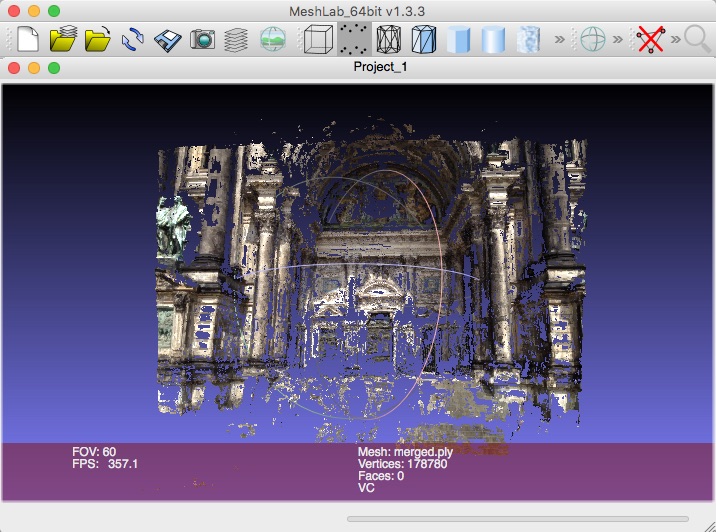
This will run dense multiview stereo matching and produce a denser point cloud stored in data/berlin/depthmaps/merged.ply. You can visualize that point cloud using MeshLab or any other viewer that supports PLY files.
For the Berlin dataset you should get something similar to this
To reconstruct your own images,
- put some images in
data/DATASET_NAME/images/, and - copy
data/berlin/config.yml` to ``data/DATASET_NAME/config.yaml
Reconstruction Commands
There are several steps required to do a 3D reconstruction including feature detection, matching, SfM reconstruction and dense matching. OpenSfM performs these steps using different commands that store the results into files for other commands to use.
The single application bin/opensfm is used to run those commands. The first argument of the application is the command to run and the second one is the dataset to run the commands on.
Here is the usage page of bin/opensfm, which lists the available commands:
usage: opensfm [-h] command ...

positional arguments:
  command            Command to run
    extract_metadata
                     Extract metadata form images' EXIF tag
    detect_features  Compute features for all images
    match_features   Match features between image pairs
    create_tracks    Link matches pair-wise matches into tracks
    reconstruct      Compute the reconstruction
    mesh             Add delaunay meshes to the reconstruction
    undistort        Save radially undistorted images
    compute_depthmaps
                     Compute depthmap
    export_ply       Export reconstruction to PLY format
    export_openmvs   Export reconstruction to openMVS format
    export_visualsfm
                     Export reconstruction to NVM_V3 format from VisualSfM

optional arguments:
  -h, --help         show this help message and exit
extract_metadata
This commands extracts EXIF metadata from the images an stores them in the exif folder and the camera_models.json file.
The following data is extracted for each image:
widthandheight: image size in pixelsgpslatitude,longitude,altitudeanddop: The GPS coordinates of the camera at capture time and the corresponding Degree Of Precission). This is used to geolocate the reconstruction.capture_time: The capture time. Used to choose candidate matching images when the optionmatching_time_neighborsis set.camera orientation: The EXIF orientation tag (see this exif orientation documentation). Used to orient the reconstruction straigh up.projection_type: The camera projection type. It is extracted from the GPano metadata and used to determine which projection to use for each camera. Supported types are perspective, equirectangular and fisheye.focal_ratio: The focal length provided by the EXIF metadata divided by the sensor width. This is used as initialization and prior for the camera focal length parameter.makeandmodel: The camera make and model. Used to build the camera ID.camera: The camera ID string. Used to identify a camera. When multiple images have the same camera ID string, they will be assumed to be taken with the same camera and will share its parameters.
Once the metadata for all images has been extracted, a list of camera models is created and stored in camera_models.json. A camera is created for each diferent camera ID string found on the images.
For each camera the following data is stored:
widthandheight: image size in pixelsprojection_type: the camera projection typefocal: The initial estimation of the focal length (as a multiple of the sensor width).k1andk2: The initial estimation of the radial distortion parameters. Only used for perspective and fisheye projection models.focal_prior: The focal length prior. The final estimated focal length will be forced to be similar to it.k1_priorandk2_prior: The radial distortion parameters prior.
Providing your own camera parameters
By default, the camera parameters are taken from the EXIF metadata but it is also possible to override the default parameters. To do so, place a file named camera_models_overrides.json in the project folder. This file should have the same structure as camera_models.json. When running the extract_metadata command, the parameters of any camera present in the camera_models_overrides.json file will be copied to camera_models.json overriding the default ones.
Simplest way to create the camera_models_overrides.json file is to rename camera_models.json and modify the parameters. You will need to rerun the extract_metadata command after that.
Here is a spherical 360 images dataset example using camera_models_overrides.json to specify that the camera is taking 360 equirectangular images.
detect_features
This command detect feature points in the images and stores them in the feature folder.
match_features
This command matches feature points between images and stores them in the matches folder. It first determines the list of image pairs to run, and then run the matching process for each pair to find corresponding feature points.
Since there are a lot of possible image pairs, the process can be very slow. It can be speeded up by restricting the list of pairs to match. The pairs can be restricted by GPS distance, capture time or file name order.
create_tracks
This command links the matches between pairs of images to build feature point tracks. The tracks are stored in the tracks.csv file. A track is a set of feature points from different images that have been recognized to correspond to the same pysical point.
reconstruct
This command runs the incremental reconstruction process. The goal of the reconstruction process is to find the 3D position of tracks (the structure) together with the position of the cameras (the motion). The computed reconstruction is stored in the reconstruction.json file.
mesh
This process computes a rough triangular mesh of the scene seen by each images. Such mesh is used for simulating smooth motions between images in the web viewer. The reconstruction with the mesh added is stored in reconstruction.meshed.json file.
Note that the only difference between reconstruction.json and reconstruction.meshed.json is that the later contains the triangular meshes. If you don’t need that, you only need the former file and there’s no need to run this command.
undistort
This command creates undistorted version of the reconstruction, tracks and images. The undistorted version can later be used for computing depth maps.
compute_depthmaps
This commands computes a dense point cloud of the scene by computing and merging depthmaps. It requires an undistorted reconstructions. The resulting depthmaps are stored in the depthmaps folder and the merged point cloud is stored in depthmaps/merged.ply
Configuration
TODO explain config.yaml and the available parameters
Ground Control Points
When EXIF data contains GPS location, it is used by OpenSfM to georeference the reconstruction. Additionally, it is possible to use ground control points.
Ground control points (GCP) are landmarks visible on the images for which the geospatial position (latitude, longitude and altitude) is known. A single GCP can be observed in one or more images.
OpenSfM uses GCP in two steps of the reconstruction process: alignment and bundle adjustment. In the alignment step, points are used to globaly move the reconstruction so that the observed GCP align with their GPS position. Two or more observations for each GCP are required for it to be used during the aligment step.
In the bundle adjustment step, GCP observations are used as a constraint to refine the reconstruction. In this step, all ground control points are used. No minimum number of observation is required.
File format
GCPs can be specified by adding a text file named gcp_list.txt at the root folder of the dataset. The format of the file should be as follows.
The first line should contain the name of the projection used for the geo coordinates.
The following lines should con should contain the data for each ground control point observation. One per line and in the format:
<geo_x> <geo_y> <geo_z> <im_x> <im_y> <image_name>
Where
<geo_x> <geo_y> <geo_z>are the geospatial coordinates of the GCP and<im_x> <im_y>are the pixel coordinates where the GCP is observed.
Supported projections
The geospatial coordinates can be specified in one the following formats.
- WGS84: This is the standard latitude, longitude coordinates used by most GPS devices. In this case,
<geo_x> = longitude,<geo_y> = latitudeand<geo_z> = altitude - UTM: UTM projections can be specified using a string projection string such as
WGS84 UTM 32N, where 32 is the region and N is . In this case,<geo_x> = E,<geo_y> = Nand<geo_z> = altitude - proj4: Any valid proj4 format string can be used. For example, for UTM 32N we can use
+proj=utm +zone=32 +north +ellps=WGS84 +datum=WGS84 +units=m +no_defs
Example
This file defines 2 GCP whose coordinates are specified in the WGS84 standard. The first one is observed in both 01.jpg and 02.jpg, while the second one is only observed in 01.jpg
WGS84
13.400740745 52.519134104 12.0792090446 2335.0 1416.7 01.jpg
13.400740745 52.519134104 12.0792090446 2639.1 938.0 02.jpg
13.400502446 52.519251158 16.7021233002 766.0 1133.1 01.jpg